CLIP FUNDAMENTALS
Topic: CLIP Contrastive Language-Image Pretraining
Author: Giordano Cicchetti
This lab shows how to implement one of the most influential frameworks of recent years in the field of multimodal learning: CLIP (Radford et al., 2021).
Here is a summary of what this lab will cover:
- General theoretical introduction
- How to implement the CLIP loss function
- How to pretrain image and text encoders using the CLIP loss function
- How to evaluate the knowledge acquired by these models
Suggested readings before starting:
!pip install open_clip_torch --quiet
import torch
import torch.nn as nn
import torch.nn.functional as F
from torchvision import transforms, datasets
from torch.utils.data import DataLoader
from tqdm import tqdm
import open_clip
from torchvision.datasets import CocoCaptions
from PIL import Image
Section 1: Theoretical introduction
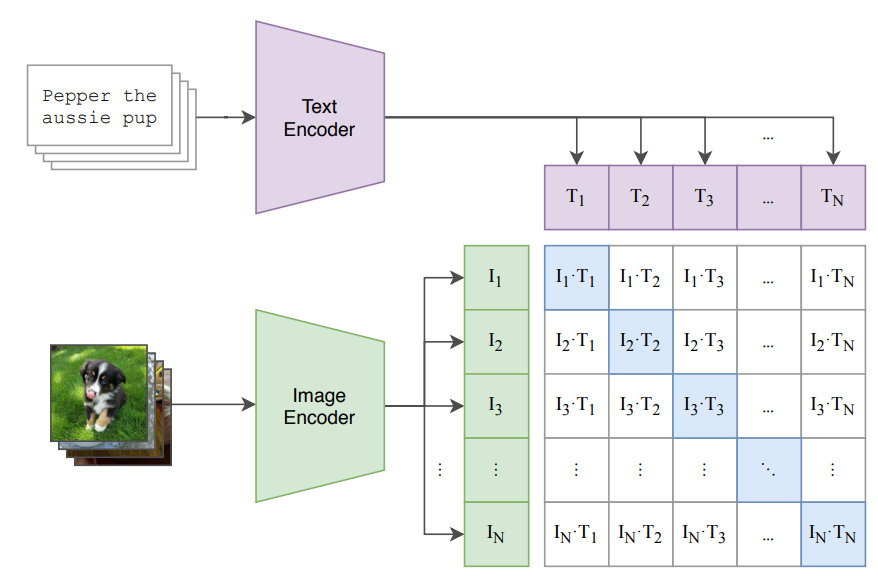
CLIP (Contrastive Language–Image Pretraining) is a framework introduced by OpenAI that learns visual representations from natural language supervision. It achieves strong zero-shot performance on a wide range of image classification tasks.
Key Ideas
- Learn a shared embedding space for text and images. Where these two modalities are connected to each other by means of semantics meaning (i.e. the embedding of the image of a dog is 'close' to the embedding of the text caption "the photo of a dog").
- Use contrastive loss to align matching image-text pairs and separate non-matching ones.
- Concepts of closeness and alignement expressed in terms of cosine similarity.
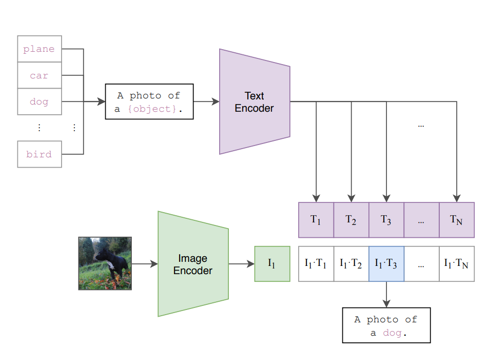
- Enables zero-shot classification without task-specific fine-tuning.
CLIP Architecture
CLIP is composed of two encoders:
- Image Encoder: Typically ResNet-50 or ViT.
- Text Encoder: Typically Transformer-based.
Both encoders project their inputs into a shared embedding space. The latent dimension of such latent space is an hyperparameter that can be choosed at design phase.
CLIP Use Case
Main use: CLIP is used to pre-train text and visual models that can be used/incorporated in downstram tasks.
Major examples are:
-
CLIP text encoder used as text conditioning module in text-to-content generation models [1-2];
-
CLIP image encoder used in Multimodal LLM to encode visual informations. [3-4]
[1] Ramesh, Aditya, et al. "Hierarchical text-conditional image generation with clip latents." arXiv preprint arXiv:2204.06125 1.2 (2022): 3.
[2] Liu, Haohe, et al. "Audioldm: Text-to-audio generation with latent diffusion models." International conference on machine learning. PMLR, 2023.
[3] Liu, Haotian, et al. "Visual instruction tuning." Advances in neural information processing systems 36 NeurIPS (2023)
[4] Li, Junnan, et al. "Blip-2: Bootstrapping language-image pre-training with frozen image encoders and large language models." International conference on machine learning. PMLR, 2023.
Diagram
Section 2: CLIP Loss Function
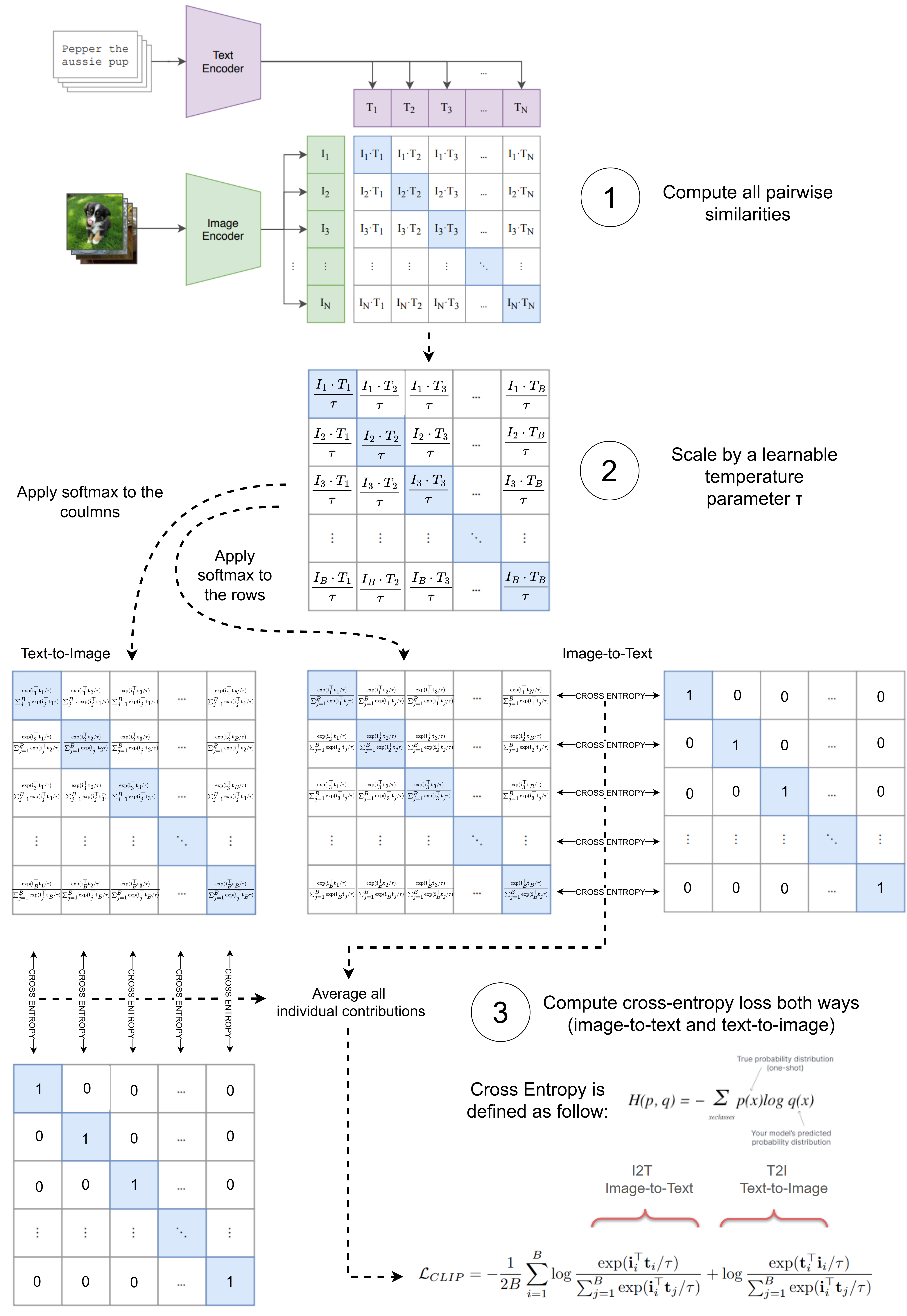
CLIP uses a symmetric cross-entropy loss based on cosine similarities. This loss encourages matching image-text pairs to have similar embeddings while pushing apart non-matching pairs.
Given a batch of N (image, text) pairs:
- Compute all pairwise similarities $S_{ij} = cosine(img_i, txt_j)$
- Scale by a learnable temperature parameter τ
- Compute cross-entropy loss both ways (image-to-text and text-to-image)
Mathematically:
\[\mathcal{L}_{\mathrm{CLIP}} = -\frac{1}{2B} \sum_{i=1}^{B} \Biggl[ \underbrace{ \log \frac{ \exp\bigl(\langle \mathbf{I}_i, \mathbf{T}_i \rangle / \tau\bigr) }{ \sum_{j=1}^{B} \exp\bigl(\langle \mathbf{I}_i, \mathbf{T}_j \rangle / \tau\bigr) } }_{\text{I2T: Image-to-Text}} \;+\; \underbrace{ \log \frac{ \exp\bigl(\langle \mathbf{T}_i, \mathbf{I}_i \rangle / \tau\bigr) }{ \sum_{j=1}^{B} \exp\bigl(\langle \mathbf{T}_i, \mathbf{I}_j \rangle / \tau\bigr) } }_{\text{T2I: Text-to-Image}} \Biggr]\]Let’s break it down into parts and analyze each component to better understand its behavior;
1) Compute all pairwise similarities
\[\begin{equation} S_{ij} = cosine(img_i, txt_j) \end{equation}\]The cosine similarity between two generic vectors $A$ and $B$ in the same dimensional space $\mathbb{R}^d$, is defined as the cosine value of the angle $\theta$ between them:
\[\begin{equation} cos(\theta)= \frac{\langle \mathbf{A}, \mathbf{B} \rangle}{||\mathbf{A}|| ||\mathbf{B}||} \end{equation}\]In the clip loss function the cosine similarity is present in the dot products \(\begin{equation} \langle \textbf{I}_i, \textbf{T}_i \rangle \end{equation}\)
The denominator?
- $\mathbf{I}_i$ and $\mathbf{T}_i$ are extracted embeddings from the image and text encoder.
- Key assumption of CLIP loss function is that $\mathbf{I}_i$ and $\mathbf{T}_i$ are vectors normalized to unitary norm. (i.e. we ALWAYS have to normalize embeddings coming out from encoders, unless explicitly defined)
- The same subscript $_i$ tell us that they corresponds to paired content with the same semantic.
i = torch.randn(1,512) # Assume this is the output of the image encoder
t = torch.randn(1,512) # Assume this is the ouput of the text encoder

print(f"The shape of i vector is {i.shape}")
print(f"The shape of t vector is {t.shape}")
The shape of i vector is torch.Size([1, 512])
The shape of t vector is torch.Size([1, 512])
# Lets Check the norm of i and t
print(f"The norm of i is {i.norm()}")
print(f"The norm of t is {t.norm()}")
The norm of i is 22.876724243164062
The norm of t is 22.4530086517334
# Normalize to unitary norm
i = F.normalize(i, p=2, dim=1)
t = F.normalize(t, p=2, dim=1)

print(f"The norm of i is {i.norm():.2f}")
print(f"The norm of t is {t.norm():.2f}")
The norm of i is 1.00
The norm of t is 1.00
Now that we have unitary norm vectors, we can compute the cosine similarity among them just with the dot product
cosine_similarity = i @ t.T # [1,512] @ [512,1] = [1,1]
print(f"The cosine similarity is {cosine_similarity.item():.2f}")
The cosine similarity is -0.04
Working with batches
Assume you have a batch of N image-text pairs:
Images → encoded as vectors $\mathbf{I}_1, \mathbf{I}_2, \cdots, \mathbf{I}_n$
Texts → encoded as vectors $\mathbf{T}_1, \mathbf{T}_2, \cdots, \mathbf{T}_n$
CLIP computes cosine similarities among all image-text combinations in the batch: \(\begin{equation} \mathbf{S}_{ ij} = ⟨\mathbf{I}_i,\mathbf{T}_j⟩ \end{equation}\)
$\mathbf{S}$ is a matrix of shape [B, B], containing similarity scores.
B = 5

i = torch.randn(B,512) # Assume this is the output of the image encoder
t = torch.randn(B,512) # Assume this is the ouput of the text encoder

# Normalize to unitary norm
i = F.normalize(i, p=2, dim=1)
t = F.normalize(t, p=2, dim=1)

S = i @ t.T   #[B,512] @ [512,B] = [B,B]
print(f"The shape of S is {S.shape}")
print(f"The shape of S is: \n{S}")
The shape of S is torch.Size([5, 5])
The shape of S is:
tensor([[ 0.0347,  0.0375, -0.0328, -0.0253, -0.0745],
        [ 0.0179,  0.0866, -0.0741, -0.0032, -0.0220],
        [-0.0151,  0.0109, -0.0295,  0.0496,  0.0703],
        [-0.0272, -0.0400, -0.0184,  0.0262,  0.0691],
        [ 0.0432, -0.0579,  0.0218, -0.0007, -0.0053]])
2) Scale by a learnable temperature parameter τ
\[\begin{equation} \mathbf{S}_{ ij} = \frac{⟨\mathbf{I}_i,\mathbf{T}_j⟩}{\tau} \end{equation}\]Effects of Temperature on Model Behavior
- Lower Temperature ($\tau$ ↓)
-
Sharper softmax distribution: Emphasizes differences between positive and negative pairs.
-
Focus on hard negatives: The model pays more attention to challenging negative samples that are similar to the positive ones.
-
Risk of over-separation: May push apart semantically similar samples that shouldn't be separated, potentially harming generalization.
- Higher Temperature ($\tau$ ↑)
-
Smoother softmax distribution: Reduces emphasis on individual pair differences.
-
Tolerance to similar negatives: Allows semantically similar samples to remain closer in the embedding space.
-
Risk of under-separation: May not sufficiently distinguish between dissimilar samples, leading to less discriminative embeddings.
Practical Considerations
-
Learnable τ: CLIP often treats τ as a learnable parameter, allowing the model to find an optimal value during training.
-
Dataset dependency: Optimal τ may vary based on dataset characteristics, such as class balance and semantic diversity.
-
Dynamic τ: Some approaches adjust τ during training to balance the focus between hard negatives and overall embedding structure.
-
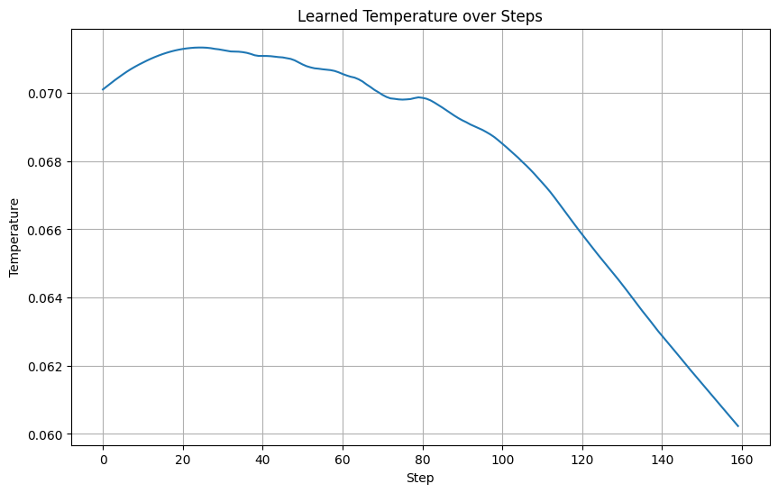
Typical temperature values range from 0.1 to 0.01. Temperature in the original CLIP paper: Learnable starting from 0.07
temperature = 0.07 #Define the temperature parameter

S_scaled = S / temperature

print(f"The shape of S_scaled is {S_scaled.shape}")
print(f"The shape of S_scaled is: \n{S_scaled}")
The shape of S_scaled is torch.Size([5, 5])
The shape of S_scaled is:
tensor([[ 0.4956,  0.5359, -0.4687, -0.3611, -1.0650],
        [ 0.2563,  1.2378, -1.0579, -0.0460, -0.3147],
        [-0.2156,  0.1557, -0.4212,  0.7079,  1.0038],
        [-0.3892, -0.5716, -0.2630,  0.3744,  0.9868],
        [ 0.6172, -0.8265,  0.3112, -0.0093, -0.0752]])
3) Compute cross-entropy loss both ways (image-to-text and text-to-image)
# Targets: index of matching pairs
targets = torch.arange(B) # [0,1,2,3....,B]

# Cross-entropy losses
loss_i2t = F.cross_entropy(S_scaled, targets)        # Image to text
loss_t2i = F.cross_entropy(S_scaled.T, targets)      # Text to image

# Final CLIP loss
loss = (loss_i2t + loss_t2i) / 2
print(f"The final CLIP loss is {loss.item():.2f}")
Code
class ClipLoss(nn.Module):
    def __init__(self, temperature=0.07):
        super().__init__()
        # Let the temperature be a learnable parameter
        self.temperature = nn.Parameter(torch.tensor(temperature))
        # Otherwise
        # self.temperature = torch.tensor(temperature)

    def forward(self, image_features, text_features):
        # image features: [B,D]
        # text features: [B,D]

        # Normalize
        image_features = F.normalize(image_features, dim=1)
        text_features = F.normalize(text_features, dim=1)

        # Similarity matrix and temperature scaling
        logits_per_image = image_features @ text_features.t() / self.temperature
        logits_per_text = text_features @ image_features.t() / self.temperature

        batch_size = image_features.size(0)
        labels = torch.arange(batch_size).to(image_features.device)

        loss_i2t = F.cross_entropy(logits_per_image, labels)
        loss_t2i = F.cross_entropy(logits_per_text, labels)

        return (loss_i2t + loss_t2i) / 2
Section 3: Training session
Load Mini-Coco Dataset
Handmade dataset from MSCOCO https://cocodataset.org/#home
1000 Image-Text pairs for training 100 Image-Text pairs for testing
Just for fun :)
!gdown 1ld44JrobUwxlSnLEncdXIqX2tCeZA-fd

!unzip /content/mini_coco.zip
Retrieval tasks:
-
Image-to-Text Retrieval (Image → Text):
Given an image as a query, the goal is to retrieve the most relevant textual descriptions (captions) from a collection. This is useful in applications like automatic image captioning or image search engines that return text results.
-
Text-to-Image Retrieval (Text → Image):
Given a text query (e.g., a sentence or phrase), the goal is to retrieve the most relevant images from a dataset. This is common in systems like search engines or content recommendation platforms where users describe what they want to see.
def compute_retrieval_metrics(x: torch.Tensor):

    sx, _ = torch.sort(-x, dim=1)
    d = torch.diagonal(-x)


    d = d.unsqueeze(1)  # Make it (N, 1)
    ind_matrix = sx - d
    matches = (ind_matrix == 0)
    ind = matches.float().argmax(dim=1)

    metrics = {
        'R1': float((ind == 0).sum().item()) * 100 / len(ind),
        'R5': float((ind < 5).sum().item()) * 100 / len(ind),
        'R10': float((ind < 10).sum().item()) * 100 / len(ind),
    }
    return metrics
Training and Validation pipeline
# --- CONFIG ---
BATCH_SIZE = 64
NUM_EPOCHS = 10
DEVICE = "cuda" if torch.cuda.is_available() else "cpu"
MODEL_NAME = "RN50"
PRETRAINED = None  # Start from scratch

# --- DATASET ---
transform = transforms.Compose([
    transforms.Resize((224, 224)),
    transforms.ToTensor(),
    transforms.Normalize((0.48145466, 0.4578275, 0.40821073),
                         (0.26862954, 0.26130258, 0.27577711)),
])


train_dataset = CocoCaptions(
    root='./mini_coco/train2017',
    annFile='./mini_coco/annotations/captions_train2017.json',
    transform=transform
)

val_dataset =  CocoCaptions(
    root='./mini_coco/val2017',
    annFile='./mini_coco/annotations/captions_val2017.json',
    transform=transform
)
def collate_fn(batch):
    images, captions = zip(*batch)
    images = torch.stack(images)
    texts = [cap[0] for cap in captions]  # use the first caption
    return images, texts

train_loader = DataLoader(train_dataset, batch_size=BATCH_SIZE, shuffle=True,
                        collate_fn=collate_fn, num_workers=4)

val_loader = DataLoader(val_dataset, batch_size=BATCH_SIZE, shuffle=False,
                        collate_fn=collate_fn, num_workers=4)

# --- MODEL ---
model, _, preprocess = open_clip.create_model_and_transforms(MODEL_NAME, pretrained=PRETRAINED)
tokenizer = open_clip.get_tokenizer(MODEL_NAME)
model = model.to(DEVICE)
loss_fn = ClipLoss(temperature=0.07)

# --- TRAINING ---
optimizer = torch.optim.Adam([x for x in model.parameters()]+[x for x in loss_fn.parameters()], lr=1e-4)

# --- TRACK FOR PLOT ---
loss_values = []
temperature_values = []


# --- TRAIN + VALIDATION ---
for epoch in range(NUM_EPOCHS):
    model.train()
    total_loss = 0

    for images, texts in tqdm(train_loader, desc=f"Epoch {epoch+1} [Training]"):
        images = images.to(DEVICE)
        texts = tokenizer(texts).to(DEVICE)

        image_features = model.encode_image(images)
        text_features = model.encode_text(texts)

        loss = loss_fn(image_features, text_features)

        optimizer.zero_grad()
        loss.backward()
        optimizer.step()

        total_loss += loss.item()
        loss_values.append(loss.item())
        temperature_values.append(loss_fn.temperature.item())

    avg_loss = total_loss / len(train_loader)
    print(f"Epoch {epoch+1} — Training Loss: {avg_loss:.4f}")

    # --- VALIDATION ---
    model.eval()
    with torch.no_grad():
        all_image_features = []
        all_text_features = []

        for images, texts in tqdm(val_loader, desc=f"Epoch {epoch+1} [Validation]"):
            images = images.to(DEVICE)
            texts = tokenizer(texts).to(DEVICE)

            image_feats = F.normalize(model.encode_image(images), dim=-1)
            text_feats = F.normalize(model.encode_text(texts), dim=-1)

            all_image_features.append(image_feats)
            all_text_features.append(text_feats)

        image_features = torch.cat(all_image_features, dim=0)
        text_features = torch.cat(all_text_features, dim=0)

        similarity = image_features @ text_features.T

        metrics_i2t = compute_retrieval_metrics(similarity)
        print(f"Validation Accuracy — Image→Text: R1 {metrics_i2t['R1']:.4f}, R5 {metrics_i2t['R5']:.4f}, R10 {metrics_i2t['R10']:.4f}")

        metrics_t2i = compute_retrieval_metrics(similarity.T)
        print(f"Validation Accuracy — Text→Image: R1 {metrics_t2i['R1']:.4f}, R5 {metrics_t2i['R5']:.4f}, R10 {metrics_t2i['R10']:.4f}")
Epoch 1 [Training]: 100%|██████████| 16/16 [00:21<00:00,  1.33s/it]

Epoch 1 — Training Loss: 4.1814

Epoch 1 [Validation]: 100%|██████████| 2/2 [00:01<00:00,  1.18it/s]
Validation Accuracy — Image→Text: R1 1.0000, R5 5.0000, R10 12.0000
Validation Accuracy — Text→Image: R1 1.0000, R5 5.0000, R10 11.0000

Epoch 2 [Training]: 100%|██████████| 16/16 [00:19<00:00,  1.20s/it]

Epoch 2 — Training Loss: 4.0629

Epoch 2 [Validation]: 100%|██████████| 2/2 [00:01<00:00,  1.25it/s]

Validation Accuracy — Image→Text: R1 3.0000, R5 6.0000, R10 15.0000
Validation Accuracy — Text→Image: R1 1.0000, R5 5.0000, R10 14.0000

Epoch 3 [Training]: 100%|██████████| 16/16 [00:19<00:00,  1.22s/it]

Epoch 3 — Training Loss: 3.7348

Epoch 3 [Validation]: 100%|██████████| 2/2 [00:01<00:00,  1.20it/s]

Validation Accuracy — Image→Text: R1 5.0000, R5 13.0000, R10 25.0000
Validation Accuracy — Text→Image: R1 3.0000, R5 12.0000, R10 21.0000

Epoch 4 [Training]: 100%|██████████| 16/16 [00:20<00:00,  1.27s/it]

Epoch 4 — Training Loss: 3.1225

Epoch 4 [Validation]: 100%|██████████| 2/2 [00:01<00:00,  1.25it/s]

Validation Accuracy — Image→Text: R1 3.0000, R5 11.0000, R10 21.0000
Validation Accuracy — Text→Image: R1 4.0000, R5 12.0000, R10 18.0000

Epoch 5 [Training]: 100%|██████████| 16/16 [00:20<00:00,  1.26s/it]

Epoch 5 — Training Loss: 2.5640

Epoch 5 [Validation]: 100%|██████████| 2/2 [00:01<00:00,  1.25it/s]

Validation Accuracy — Image→Text: R1 3.0000, R5 14.0000, R10 27.0000
Validation Accuracy — Text→Image: R1 1.0000, R5 13.0000, R10 26.0000

Epoch 6 [Training]: 100%|██████████| 16/16 [00:20<00:00,  1.25s/it]

Epoch 6 — Training Loss: 1.9938

Epoch 6 [Validation]: 100%|██████████| 2/2 [00:01<00:00,  1.04it/s]

Validation Accuracy — Image→Text: R1 5.0000, R5 12.0000, R10 17.0000
Validation Accuracy — Text→Image: R1 3.0000, R5 11.0000, R10 18.0000

Epoch 7 [Training]: 100%|██████████| 16/16 [00:20<00:00,  1.29s/it]

Epoch 7 — Training Loss: 1.5335

Epoch 7 [Validation]: 100%|██████████| 2/2 [00:01<00:00,  1.27it/s]

Validation Accuracy — Image→Text: R1 6.0000, R5 18.0000, R10 25.0000
Validation Accuracy — Text→Image: R1 2.0000, R5 13.0000, R10 26.0000

Epoch 8 [Training]: 100%|██████████| 16/16 [00:20<00:00,  1.30s/it]

Epoch 8 — Training Loss: 1.0845

Epoch 8 [Validation]: 100%|██████████| 2/2 [00:01<00:00,  1.25it/s]

Validation Accuracy — Image→Text: R1 4.0000, R5 16.0000, R10 26.0000
Validation Accuracy — Text→Image: R1 5.0000, R5 17.0000, R10 27.0000

Epoch 9 [Training]: 100%|██████████| 16/16 [00:20<00:00,  1.28s/it]

Epoch 9 — Training Loss: 0.8292

Epoch 9 [Validation]: 100%|██████████| 2/2 [00:01<00:00,  1.12it/s]

Validation Accuracy — Image→Text: R1 4.0000, R5 17.0000, R10 28.0000
Validation Accuracy — Text→Image: R1 1.0000, R5 16.0000, R10 24.0000

Epoch 10 [Training]: 100%|██████████| 16/16 [00:20<00:00,  1.27s/it]

Epoch 10 — Training Loss: 0.6429

Epoch 10 [Validation]: 100%|██████████| 2/2 [00:01<00:00,  1.25it/s]

Validation Accuracy — Image→Text: R1 6.0000, R5 17.0000, R10 28.0000
Validation Accuracy — Text→Image: R1 4.0000, R5 20.0000, R10 26.0000
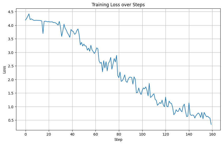
# Plot all the values inside loss_values array and temperature_values

import matplotlib.pyplot as plt

plt.figure(figsize=(10, 6))
plt.plot(loss_values)
plt.title('Training Loss over Steps')
plt.xlabel('Step')
plt.ylabel('Loss')
plt.grid(True)
plt.show()

plt.figure(figsize=(10, 6))
plt.plot(temperature_values)
plt.title('Learned Temperature over Steps')
plt.xlabel('Step')
plt.ylabel('Temperature')
plt.grid(True)
plt.show()
Section 4: Validation session
OpenCLIP library, is an open source reimplementation of OpenAI’s CLIP (Contrastive Language-Image Pre-training) model. It provides a flexible and scalable codebase that allows researchers and developers to train, fine-tune, and deploy CLIP models on various datasets and hardware configurations.
import open_clip

available_models = open_clip.list_pretrained()

for model_name, pretrained_dataset in available_models:
    print(f"Model: {model_name}, Pretrained on: {pretrained_dataset}")
Model: RN50, Pretrained on: openai
Model: RN50, Pretrained on: yfcc15m
Model: RN50, Pretrained on: cc12m
Model: RN101, Pretrained on: openai
Model: RN101, Pretrained on: yfcc15m
Model: RN50x4, Pretrained on: openai
Model: RN50x16, Pretrained on: openai
Model: RN50x64, Pretrained on: openai
Model: ViT-B-32, Pretrained on: openai
Model: ViT-B-32, Pretrained on: laion400m_e31
Model: ViT-B-32, Pretrained on: laion400m_e32
Model: ViT-B-32, Pretrained on: laion2b_e16
Model: ViT-B-32, Pretrained on: laion2b_s34b_b79k
Model: ViT-B-32, Pretrained on: datacomp_xl_s13b_b90k
Model: ViT-B-32, Pretrained on: datacomp_m_s128m_b4k
Model: ViT-B-32, Pretrained on: commonpool_m_clip_s128m_b4k
Model: ViT-B-32, Pretrained on: commonpool_m_laion_s128m_b4k
Model: ViT-B-32, Pretrained on: commonpool_m_image_s128m_b4k
Model: ViT-B-32, Pretrained on: commonpool_m_text_s128m_b4k
Model: ViT-B-32, Pretrained on: commonpool_m_basic_s128m_b4k
Model: ViT-B-32, Pretrained on: commonpool_m_s128m_b4k
Model: ViT-B-32, Pretrained on: datacomp_s_s13m_b4k
Model: ViT-B-32, Pretrained on: commonpool_s_clip_s13m_b4k
Model: ViT-B-32, Pretrained on: commonpool_s_laion_s13m_b4k
Model: ViT-B-32, Pretrained on: commonpool_s_image_s13m_b4k
Model: ViT-B-32, Pretrained on: commonpool_s_text_s13m_b4k
Model: ViT-B-32, Pretrained on: commonpool_s_basic_s13m_b4k
Model: ViT-B-32, Pretrained on: commonpool_s_s13m_b4k
Model: ViT-B-32, Pretrained on: metaclip_400m
Model: ViT-B-32, Pretrained on: metaclip_fullcc
Model: ViT-B-32-256, Pretrained on: datacomp_s34b_b86k
Model: ViT-B-16, Pretrained on: openai
Model: ViT-B-16, Pretrained on: laion400m_e31
Model: ViT-B-16, Pretrained on: laion400m_e32
Model: ViT-B-16, Pretrained on: laion2b_s34b_b88k
Model: ViT-B-16, Pretrained on: datacomp_xl_s13b_b90k
Model: ViT-B-16, Pretrained on: datacomp_l_s1b_b8k
Model: ViT-B-16, Pretrained on: commonpool_l_clip_s1b_b8k
Model: ViT-B-16, Pretrained on: commonpool_l_laion_s1b_b8k
Model: ViT-B-16, Pretrained on: commonpool_l_image_s1b_b8k
Model: ViT-B-16, Pretrained on: commonpool_l_text_s1b_b8k
Model: ViT-B-16, Pretrained on: commonpool_l_basic_s1b_b8k
Model: ViT-B-16, Pretrained on: commonpool_l_s1b_b8k
Model: ViT-B-16, Pretrained on: dfn2b
Model: ViT-B-16, Pretrained on: metaclip_400m
Model: ViT-B-16, Pretrained on: metaclip_fullcc
Model: ViT-B-16-plus-240, Pretrained on: laion400m_e31
Model: ViT-B-16-plus-240, Pretrained on: laion400m_e32
Model: ViT-L-14, Pretrained on: openai
Model: ViT-L-14, Pretrained on: laion400m_e31
Model: ViT-L-14, Pretrained on: laion400m_e32
Model: ViT-L-14, Pretrained on: laion2b_s32b_b82k
Model: ViT-L-14, Pretrained on: datacomp_xl_s13b_b90k
Model: ViT-L-14, Pretrained on: commonpool_xl_clip_s13b_b90k
Model: ViT-L-14, Pretrained on: commonpool_xl_laion_s13b_b90k
Model: ViT-L-14, Pretrained on: commonpool_xl_s13b_b90k
Model: ViT-L-14, Pretrained on: metaclip_400m
Model: ViT-L-14, Pretrained on: metaclip_fullcc
Model: ViT-L-14, Pretrained on: dfn2b
Model: ViT-L-14, Pretrained on: dfn2b_s39b
Model: ViT-L-14-336, Pretrained on: openai
Model: ViT-H-14, Pretrained on: laion2b_s32b_b79k
Model: ViT-H-14, Pretrained on: metaclip_fullcc
Model: ViT-H-14, Pretrained on: metaclip_altogether
Model: ViT-H-14, Pretrained on: dfn5b
Model: ViT-H-14-378, Pretrained on: dfn5b
Model: ViT-g-14, Pretrained on: laion2b_s12b_b42k
Model: ViT-g-14, Pretrained on: laion2b_s34b_b88k
Model: ViT-bigG-14, Pretrained on: laion2b_s39b_b160k
Model: ViT-bigG-14, Pretrained on: metaclip_fullcc
Model: roberta-ViT-B-32, Pretrained on: laion2b_s12b_b32k
Model: xlm-roberta-base-ViT-B-32, Pretrained on: laion5b_s13b_b90k
Model: xlm-roberta-large-ViT-H-14, Pretrained on: frozen_laion5b_s13b_b90k
Model: convnext_base, Pretrained on: laion400m_s13b_b51k
Model: convnext_base_w, Pretrained on: laion2b_s13b_b82k
Model: convnext_base_w, Pretrained on: laion2b_s13b_b82k_augreg
Model: convnext_base_w, Pretrained on: laion_aesthetic_s13b_b82k
Model: convnext_base_w_320, Pretrained on: laion_aesthetic_s13b_b82k
Model: convnext_base_w_320, Pretrained on: laion_aesthetic_s13b_b82k_augreg
Model: convnext_large_d, Pretrained on: laion2b_s26b_b102k_augreg
Model: convnext_large_d_320, Pretrained on: laion2b_s29b_b131k_ft
Model: convnext_large_d_320, Pretrained on: laion2b_s29b_b131k_ft_soup
Model: convnext_xxlarge, Pretrained on: laion2b_s34b_b82k_augreg
Model: convnext_xxlarge, Pretrained on: laion2b_s34b_b82k_augreg_rewind
Model: convnext_xxlarge, Pretrained on: laion2b_s34b_b82k_augreg_soup
Model: coca_ViT-B-32, Pretrained on: laion2b_s13b_b90k
Model: coca_ViT-B-32, Pretrained on: mscoco_finetuned_laion2b_s13b_b90k
Model: coca_ViT-L-14, Pretrained on: laion2b_s13b_b90k
Model: coca_ViT-L-14, Pretrained on: mscoco_finetuned_laion2b_s13b_b90k
Model: EVA01-g-14, Pretrained on: laion400m_s11b_b41k
Model: EVA01-g-14-plus, Pretrained on: merged2b_s11b_b114k
Model: EVA02-B-16, Pretrained on: merged2b_s8b_b131k
Model: EVA02-L-14, Pretrained on: merged2b_s4b_b131k
Model: EVA02-L-14-336, Pretrained on: merged2b_s6b_b61k
Model: EVA02-E-14, Pretrained on: laion2b_s4b_b115k
Model: EVA02-E-14-plus, Pretrained on: laion2b_s9b_b144k
Model: ViT-B-16-SigLIP, Pretrained on: webli
Model: ViT-B-16-SigLIP-256, Pretrained on: webli
Model: ViT-B-16-SigLIP-i18n-256, Pretrained on: webli
Model: ViT-B-16-SigLIP-384, Pretrained on: webli
Model: ViT-B-16-SigLIP-512, Pretrained on: webli
Model: ViT-L-16-SigLIP-256, Pretrained on: webli
Model: ViT-L-16-SigLIP-384, Pretrained on: webli
Model: ViT-SO400M-14-SigLIP, Pretrained on: webli
Model: ViT-SO400M-16-SigLIP-i18n-256, Pretrained on: webli
Model: ViT-SO400M-14-SigLIP-378, Pretrained on: webli
Model: ViT-SO400M-14-SigLIP-384, Pretrained on: webli
Model: ViT-B-32-SigLIP2-256, Pretrained on: webli
Model: ViT-B-16-SigLIP2, Pretrained on: webli
Model: ViT-B-16-SigLIP2-256, Pretrained on: webli
Model: ViT-B-16-SigLIP2-384, Pretrained on: webli
Model: ViT-B-16-SigLIP2-512, Pretrained on: webli
Model: ViT-L-16-SigLIP2-256, Pretrained on: webli
Model: ViT-L-16-SigLIP2-384, Pretrained on: webli
Model: ViT-L-16-SigLIP2-512, Pretrained on: webli
Model: ViT-SO400M-14-SigLIP2, Pretrained on: webli
Model: ViT-SO400M-14-SigLIP2-378, Pretrained on: webli
Model: ViT-SO400M-16-SigLIP2-256, Pretrained on: webli
Model: ViT-SO400M-16-SigLIP2-384, Pretrained on: webli
Model: ViT-SO400M-16-SigLIP2-512, Pretrained on: webli
Model: ViT-gopt-16-SigLIP2-256, Pretrained on: webli
Model: ViT-gopt-16-SigLIP2-384, Pretrained on: webli
Model: ViT-L-14-CLIPA, Pretrained on: datacomp1b
Model: ViT-L-14-CLIPA-336, Pretrained on: datacomp1b
Model: ViT-H-14-CLIPA, Pretrained on: datacomp1b
Model: ViT-H-14-CLIPA-336, Pretrained on: laion2b
Model: ViT-H-14-CLIPA-336, Pretrained on: datacomp1b
Model: ViT-bigG-14-CLIPA, Pretrained on: datacomp1b
Model: ViT-bigG-14-CLIPA-336, Pretrained on: datacomp1b
Model: nllb-clip-base, Pretrained on: v1
Model: nllb-clip-large, Pretrained on: v1
Model: nllb-clip-base-siglip, Pretrained on: v1
Model: nllb-clip-base-siglip, Pretrained on: mrl
Model: nllb-clip-large-siglip, Pretrained on: v1
Model: nllb-clip-large-siglip, Pretrained on: mrl
Model: MobileCLIP-S1, Pretrained on: datacompdr
Model: MobileCLIP-S2, Pretrained on: datacompdr
Model: MobileCLIP-B, Pretrained on: datacompdr
Model: MobileCLIP-B, Pretrained on: datacompdr_lt
Model: ViTamin-S, Pretrained on: datacomp1b
Model: ViTamin-S-LTT, Pretrained on: datacomp1b
Model: ViTamin-B, Pretrained on: datacomp1b
Model: ViTamin-B-LTT, Pretrained on: datacomp1b
Model: ViTamin-L, Pretrained on: datacomp1b
Model: ViTamin-L-256, Pretrained on: datacomp1b
Model: ViTamin-L-336, Pretrained on: datacomp1b
Model: ViTamin-L-384, Pretrained on: datacomp1b
Model: ViTamin-L2, Pretrained on: datacomp1b
Model: ViTamin-L2-256, Pretrained on: datacomp1b
Model: ViTamin-L2-336, Pretrained on: datacomp1b
Model: ViTamin-L2-384, Pretrained on: datacomp1b
Model: ViTamin-XL-256, Pretrained on: datacomp1b
Model: ViTamin-XL-336, Pretrained on: datacomp1b
Model: ViTamin-XL-384, Pretrained on: datacomp1b
Model: RN50-quickgelu, Pretrained on: openai
Model: RN50-quickgelu, Pretrained on: yfcc15m
Model: RN50-quickgelu, Pretrained on: cc12m
Model: RN101-quickgelu, Pretrained on: openai
Model: RN101-quickgelu, Pretrained on: yfcc15m
Model: RN50x4-quickgelu, Pretrained on: openai
Model: RN50x16-quickgelu, Pretrained on: openai
Model: RN50x64-quickgelu, Pretrained on: openai
Model: ViT-B-32-quickgelu, Pretrained on: openai
Model: ViT-B-32-quickgelu, Pretrained on: laion400m_e31
Model: ViT-B-32-quickgelu, Pretrained on: laion400m_e32
Model: ViT-B-32-quickgelu, Pretrained on: metaclip_400m
Model: ViT-B-32-quickgelu, Pretrained on: metaclip_fullcc
Model: ViT-B-16-quickgelu, Pretrained on: openai
Model: ViT-B-16-quickgelu, Pretrained on: dfn2b
Model: ViT-B-16-quickgelu, Pretrained on: metaclip_400m
Model: ViT-B-16-quickgelu, Pretrained on: metaclip_fullcc
Model: ViT-L-14-quickgelu, Pretrained on: openai
Model: ViT-L-14-quickgelu, Pretrained on: metaclip_400m
Model: ViT-L-14-quickgelu, Pretrained on: metaclip_fullcc
Model: ViT-L-14-quickgelu, Pretrained on: dfn2b
Model: ViT-L-14-336-quickgelu, Pretrained on: openai
Model: ViT-H-14-quickgelu, Pretrained on: metaclip_fullcc
Model: ViT-H-14-quickgelu, Pretrained on: dfn5b
Model: ViT-H-14-378-quickgelu, Pretrained on: dfn5b
Model: ViT-bigG-14-quickgelu, Pretrained on: metaclip_fullcc
Check out here:
https://github.com/mlfoundations/open_clip/blob/main/docs/openclip_retrieval_results.csv
https://github.com/mlfoundations/open_clip/blob/main/docs/openclip_classification_results.csv
Load a pretrained model from OpenCLIP:
model_name = 'ViT-SO400M-14-SigLIP-384'
model_pretrained, _, preprocess = open_clip.create_model_and_transforms(
    model_name, pretrained='webli'
)
tokenizer = open_clip.get_tokenizer(model_name)
model_pretrained = model_pretrained.to(DEVICE).eval()
Evaluate the performance of pretrained model on the vanilla provided test dataset:
# --- DATASET ---

val_dataset =  CocoCaptions(
    root='./mini_coco/val2017',
    annFile='./mini_coco/annotations/captions_val2017.json',
    transform=preprocess)


val_loader = DataLoader(val_dataset, batch_size=BATCH_SIZE, shuffle=False,
                        collate_fn=collate_fn, num_workers=4)

# --- VALIDATION ---
model_pretrained.eval()
with torch.no_grad():
    all_image_features = []
    all_text_features = []

    for images, texts in tqdm(val_loader, desc=f"[Validation]"):
        images = images.to(DEVICE)
        texts = tokenizer(texts).to(DEVICE)

        image_feats = F.normalize(model_pretrained.encode_image(images), dim=-1)
        text_feats = F.normalize(model_pretrained.encode_text(texts), dim=-1)

        all_image_features.append(image_feats)
        all_text_features.append(text_feats)

    image_features = torch.cat(all_image_features, dim=0)
    text_features = torch.cat(all_text_features, dim=0)
    similarity = image_features @ text_features.T

    metrics_i2t = compute_retrieval_metrics(similarity)
    print(f"Validation Accuracy — Image→Text: R1 {metrics_i2t['R1']:.2f}, R5 {metrics_i2t['R5']:.2f}, R10 {metrics_i2t['R10']:.2f}")
    metrics_t2i = compute_retrieval_metrics(similarity.T)
    print(f"Validation Accuracy — Text→Image: R1 {metrics_t2i['R1']:.2f}, R5 {metrics_t2i['R5']:.2f}, R10 {metrics_t2i['R10']:.2f}")
[Validation]: 100%|██████████| 2/2 [00:15<00:00,  7.70s/it]

Validation Accuracy — Image→Text: R1 92.00, R5 100.00, R10 100.00
Validation Accuracy — Text→Image: R1 88.00, R5 99.00, R10 100.00
Feel free to test different pretrained models.
Section 5: Zero-Shot Image Classification
In this section we will test the ability of CLIP pretrained encoders in a typical downstream task: Zero-Shot Image Classification.
CIFAR10 test dataset could be used for this purpose. It contains 10k test images with 10 testing labels: "airplane", "automobile", "bird", "cat", "deer", "dog", "frog", "horse", "ship" and "truck"
Load the CLIP pretrained encoders (we know how to do it).
# Load the model and preprocessing
model_name = "ViT-B-32"
pretrained = "openai"
device = "cuda" if torch.cuda.is_available() else "cpu"

model_pretrained, _, preprocess = open_clip.create_model_and_transforms(model_name, pretrained=pretrained)
tokenizer = open_clip.get_tokenizer(model_name)
model_pretrained = model_pretrained.to(device).eval()
Load the test dataset.
from torchvision.datasets import CIFAR10
# Load CIFAR-10 test set
cifar10_labels = [
    "airplane", "automobile", "bird", "cat", "deer",
    "dog", "frog", "horse", "ship", "truck"
]
transform = preprocess  # Use OpenCLIP's default preprocess
testset = CIFAR10(root="./data", train=False, download=True, transform=transform)
testloader = DataLoader(testset, batch_size=16, shuffle=False)
Extract Text Embeddings, one for each label.
# Tokenize class names and extract embeddings
text_inputs = tokenizer([f"a photo of a {label}" for label in cifar10_labels]).to(device)
with torch.no_grad():
    text_features = model_pretrained.encode_text(text_inputs)
    text_features = F.normalize(text_features, dim=-1)
Extract all the image embeddings and for each image embedding compute the cosine similarity score between itself and all the text embeddings. The predicted label for a given input image will be the item with the highest similarity score.
# Classify each sample in the test set
all_preds = []
all_targets = []
with torch.no_grad():
    for images, targets in tqdm(testloader):
        images = images.to(device)
        image_features = model.encode_image(images)
        image_features /= image_features.norm(dim=-1, keepdim=True)

        logits = image_features @ text_features.T
        preds = torch.argmax(logits, dim=1)

        all_preds.extend(preds.cpu().numpy())
        all_targets.extend(targets.cpu().numpy())
Compute classification metrics
from sklearn.metrics import classification_report, accuracy_score

acc = accuracy_score(all_targets, all_preds)
report = classification_report(all_targets, all_preds, target_names=cifar10_labels, digits=4)

print(f"\n Zero-Shot Image Classification Accuracy on CIFAR-10: {acc*100:.2f}%")
print("\n Detailed Classification Report:\n")
print(report)
 Zero-Shot Image Classification Accuracy on CIFAR-10: 86.17%

 Detailed Classification Report:

              precision    recall  f1-score   support

    airplane     0.9807    0.8110    0.8878      1000
  automobile     0.9768    0.8420    0.9044      1000
        bird     0.7494    0.8730    0.8065      1000
         cat     0.8565    0.7340    0.7905      1000
        deer     0.8070    0.8570    0.8312      1000
         dog     0.8138    0.8740    0.8428      1000
        frog     0.9529    0.7080    0.8124      1000
       horse     0.8140    0.9670    0.8839      1000
        ship     0.9179    0.9730    0.9447      1000
       truck     0.8417    0.9780    0.9047      1000

    accuracy                         0.8617     10000
   macro avg     0.8710    0.8617    0.8609     10000
weighted avg     0.8710    0.8617    0.8609     10000